
by Nick Colley, Senior Consulting Petrophysicist, OPC
In June, Nick Colley provided an Introduction to Petrophysics, and this article goes on to explain Petrophysics in more detail and describes how one or two of the petrophysical products are constructed.
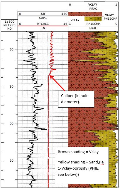
Some of the petrophysical calculations can be made in several ways, particularly for porosity and water saturation. However, considering first the clay volume estimation, this is frequently (but not always) done with the Gamma Ray (GR) log, the petrophysicist using his judgement to setting values of the GR which he deems to be 100% clay (GRMAX), and 0% clay (GRMIN). It should be noted that these values will change with depth and each formation will be likely to have different values for these two parameters.
At any depth, therefore, the clay volume (Vclay) can be computed thus:

The result would look like this:
Moving on to a consideration of porosity, the velocity of sound and its dependence on porosity was mentioned earlier. For that, we have the sonic log. There is also a tool which measures the density of the rocks: the density log – the lower the density, then in principle, the higher the porosity

|
The simplest equation to compute the water content (Sw) is the Archie equation – which applies to formations with no clay, and which have a continuous, connected pore network (a significant number of limestone formations do not have such a well-connected pore network), and which are water-wet – ie the pore network is lined with a continuous aqueous phase – again, some carbonate reservoirs are considered to be at least partly oil-wet ie the oil forms the fluid phase in contact with the rock surface (oil-wet sandstones are considered to be much less common):
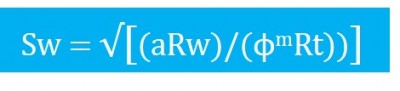
Where a and m are ‘variable constants’, usually (but by no means always) with values of 1.0 and 2.0 respectively, Rt = formation resistivity (another log), and f is porosity. The root value (known as n) is not always 2 – ie it is not necessarily the square root. It can be determined (like a and m) experimentally on core samples, and this author has seen values of reasonable reliability varying from 1.5 to ca.3 (for oil-wet samples). Rw = formation brine resistivity ie a measure of the salinity.
If the formation under investigation contains clay (they nearly always do), then modifications to the above equation are required. A number of such modified forms exist, all empirical, and the resulting equations are quite cumbersome.
Moving on to formation pressure measurement and fluid characterisation, we have Schlumberger’s MDT tool (modular dynamics tool), Baker’s RCI and Halliburton’s RDT. Pressure measurements are made at depths determined by the petrophysicist and plotted against depth. The gradient of the trend is a function of fluid density. Therefore it is clearly feasible to differentiate oil from water from gas, since gas is less dense than oil which, in turn, is less dense than water:
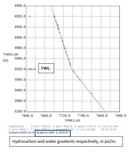
The plot above demonstrates the results from an MDT pressure survey in a reservoir containing a ‘wet’ gas with a gradient of 0.5693 psi/m (equivalent to a density of 0.4 gms/cm3), above quite a fresh (low salinity) aquifer with a pressure gradient of 1.3452 psi/m (0.95 gms/cm3). Where the two gradients intersect is the free water level (FWL), in this case 5020.3m TVDSS.
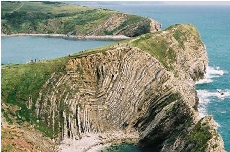
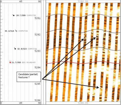
Considering now reservoir architecture, the wellbore imaging tools in the industry’s wireline inventory are used to facilitate dip computations, fracturing (if any) and sedimentology. There are two types of tool – tools which work with formation resistivity, and tools which work on the acoustic principle. The tools which use resistivity are pad-type tools and hence cannot give 100% coverage of the wellbore. Acoustic tools use a rotating transducer and hence can cover 100% of the wellbore. When the (cylindrical) image is unwrapped, the bedding can be seen as sinusoids. As long as the exact absolute orientation of the tool is known – which it is, thanks to the orientation module, loaded with inclinometers, magnetometers and accelerometers – then with suitable software, the true dip and azimuth of the geological features can be determined.
A real worked example of a resistivity image over a short section from the 12.25” section of a vertical well in Mesozoic carbonates is shown below. The right-hand half of the display is the same as the left hand side, except it has been manipulated to enhance the contrast. The red and black tadpoles show the bedding is fairly steeply dipping at ca.30 degrees to the north west (not all features have been picked, here). The bright (white = resistive) features arrowed are steeply-dipping and may be (partial ?) fractures. However, they seem to be incompletely imaged, and difficult to define completely.
To conclude:
This article has shown examples of how the Vclay, porosity (phi), water saturation (Sw), and dips can be calculated. With respect to Vclay, phi and Sw, they are by no means the only methods, but hopefully they serve to give an insight into what, and how, the petrophysicist contributes to the gas that cooks your meals, and the fuel that powers the trucks which deliver your dinner to your local (super)market.
The next step is to explain how the petrophysicist judges how much of a reservoir should be considered to be economically significant ie how much is net pay.
 Dr. Nick Colley is an expert in the Petrophysical interpretation of clastics and carbonates, and the integration of Petrophysical core analysis data. He has worked on reservoirs around the world from Trinidad to Australia via the UK, Norway, India, Libya, Nigeria, Palestine, Brazil, Bolivia, Kazakhstan and the East Indies. He worked for BG Group for more than 30 years and is now supporting OPC to develop the petrophysics service.